Enzyme Kinetics: From Rate Laws to Inhibition

Author: Polar Glacier

Reviewer: Weiming

  Note: This is a long article, and parts of it may be challenging. Students, interested readers, and people working in related fields will find a thorough treatment of the subject here.

I. Common Rate Laws in Chemical Kinetics

  Before turning to enzymes, let us review several common types of chemical reaction kinetics.

1. First-order reactions

  In a first-order reaction, the rate is directly proportional to the concentration of a reactant.

  The reaction is shown below:

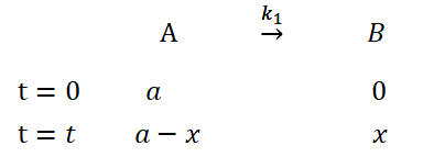
  Its rate equation can therefore be written as:

  From the definition of a first-order reaction:

  Therefore:

  Rearranging:

  Solving gives:

2. Second-order reactions

  In a second-order reaction, the rate is proportional to the square of a reactant concentration. A typical form is:

  For the reaction:

  At any point during the reaction:

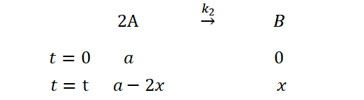
  The rate equation is:

  Combining the equations gives:

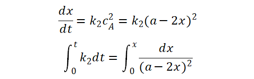
  Solving gives:

  For the reaction:

  There are two cases. If reactants A and B have the same initial concentration, the derivation is essentially the same as above and gives:

  If A and B have different initial concentrations:

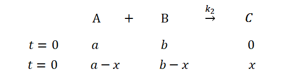
  Therefore:

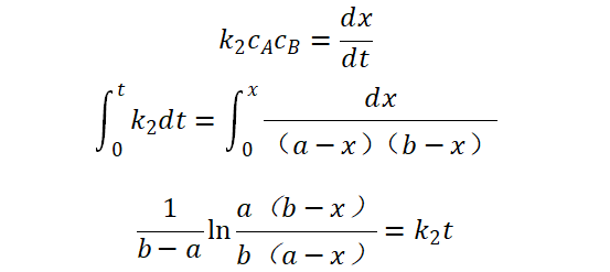
  Rate laws for reactions of integer order three or greater can be derived in much the same way as the simple second-order case.

3. Zero-order reactions

  A zero-order reaction proceeds at a constant rate independent of reactant concentration. These reactions are uncommon, but some surface reactions are zero order. One example is the decomposition of ammonia on a tungsten or iron catalyst.

  When reactant molecules adsorb to a solid catalyst at a concentration high enough to cover its surface completely, the rate depends on the available surface area rather than the reactant concentration.

  The rate equation can be written as:

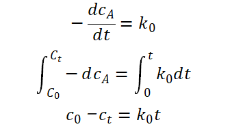
  With those basic equations reviewed, we can turn to enzyme kinetics.

II. The Intermediate-Complex Hypothesis and the Michaelis–Menten Equation

  People had long observed that chemical reactions generally speed up as reactant concentrations rise. In 1903, Victor Henri of the Sorbonne in Paris studied the hydrolysis of sucrose by invertase. He held the enzyme concentration constant, varied the sucrose concentration, and observed a rectangular hyperbola, the familiar curve found in secondary-school textbooks:

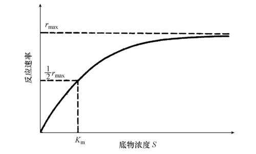
  At very low substrate concentrations, the rate rises sharply in direct proportion to substrate concentration, giving first-order behavior. As the concentration increases, the rate continues to rise but no longer proportionally. Eventually it reaches a plateau and becomes independent of substrate concentration, giving zero-order behavior. At that point, the enzyme is saturated. All enzymes show substrate saturation, although the concentration required varies.

  From these results, Henri proposed that an enzyme and its substrate combine to form an unstable intermediate on the way to product. The intermediate forms readily, then breaks down to release the product and regenerate the enzyme. This became known as the intermediate-complex hypothesis. Henri also proposed a preliminary equation for the invertase reaction:

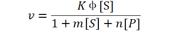
  Here K, Φ, m, and n are constants, v is the reaction rate, [S] is the substrate concentration, and [P] is the product concentration.

  In modern terms, this equation describes a substrate-inhibited enzyme reaction.

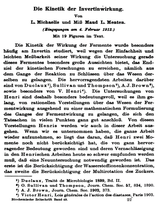
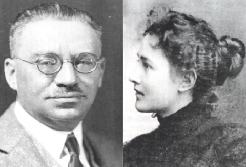
  In 1913, L. Michaelis and M. Menten revisited Henri’s results. Building on the intermediate-complex hypothesis, they treated the first step as a rapid equilibrium, derived a new mathematical expression, and published their work in Biochemische Zeitschrift (the Journal of Biochemistry, a predecessor of the FEBS Journal).

  Their rapid-equilibrium model for a single-substrate reaction can be written as:

  Here E denotes free enzyme, S the substrate, ES the unstable enzyme–substrate complex, and P the product.

Michaelis (left) and Menten (right)

  From this model, they obtained the rate law for an irreversible, single-substrate enzyme reaction: the Michaelis–Menten equation.

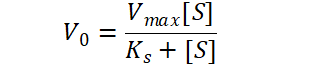
  Here V₀ is the initial rate, V_max the maximum rate, [S] the substrate concentration, and K_s the dissociation constant, equal to K₂/K₁.

  The derivation of the Michaelis–Menten equation rests on three assumptions:

• (1) At the start of the reaction, so little product has formed that the reverse reaction can be ignored.

• (2) Substrate is present at a much higher concentration than free enzyme, so its concentration remains approximately constant during the reaction.

• (3) The second step is rate-limiting, with K₂ ≫ K₃, so conversion of ES to P is too slow to disrupt the equilibrium between E and ES.

  The derivation proceeds as follows:

  Assume that E + S → ES reaches equilibrium rapidly and that the second step is much slower. The second step then determines the overall rate:

  Because [ES] is low, transient, and difficult to measure directly, we express it in terms of quantities that are easier to determine. For dissociation of ES into E and S during the rapid first-step equilibrium, the rate constant is:

  Thus:

  Because the total enzyme concentration remains constant, the enzyme mass balance is:

  Therefore:

  Substitute the preceding expression into

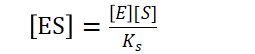
  to obtain:

  Rearranging gives:

  Substitute

  into the preceding equation to obtain:

  The maximum rate is reached when every enzyme molecule is bound to substrate. Therefore:

  Substitution gives:

  Although this model marked a major advance in enzyme kinetics, its assumptions do not apply universally. There is no reason to expect K₂ ≫ K₃ in every enzyme-catalyzed reaction, and the model does not allow the second step to be reversible. In 1925, G. E. Briggs and J. B. S. Haldane revised the Michaelis–Menten model and introduced the steady-state treatment.

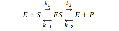
  The Briggs–Haldane steady-state treatment makes the following assumptions:

• (1) At the beginning of the reaction, product concentration is extremely low. The reverse reaction from E + P to ES is therefore negligible and can be ignored.

• (2) Initially, substrate concentration is much greater than enzyme concentration and can be treated as constant over the early part of the reaction.

• (3) Within a few milliseconds, [ES] reaches an approximately constant level. Although the concentrations of S and P continue to change, the formation rate v_f and breakdown rate v_d of ES remain nearly equal for a time, so its net rate of formation is approximately zero.

  The mathematical derivation is as follows:

  The formation rate v_f of the enzyme–substrate complex ES is:

  The breakdown rate v_d of ES is:

  At steady state, [ES] remains constant and v_f = v_d:

  From the enzyme mass balance

  we obtain:

  Substitution gives:

  Rearranging gives:

  Let:

  Then:

  Solving for [ES] gives:

  Substitute this into

  to obtain:

  The steady-state and rapid-equilibrium models lead to equations of the same form, but the steady-state treatment is more general. Both are known as the Michaelis–Menten equation, and K_m is called the Michaelis constant.

  Now let us return to Henri’s graph.

  A simple calculation shows that:

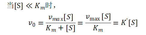
  The rate is proportional to the first power of substrate concentration, so the reaction is first order.

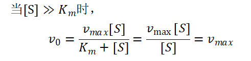
  The rate is constant, so the reaction is zero order.

  When substrate concentration lies between 0.01K_m and 100K_m, the rate follows the full Michaelis–Menten equation and the reaction is of mixed order.

  This agrees with the experimental results.

  When [S] = K_m,

  the Michaelis constant is the substrate concentration at which the reaction proceeds at half its maximum rate.

III. The Michaelis Constant

  The Michaelis constant has several other useful interpretations:

• (1) It is an important quantity in enzymology. From the derivation of K_m:

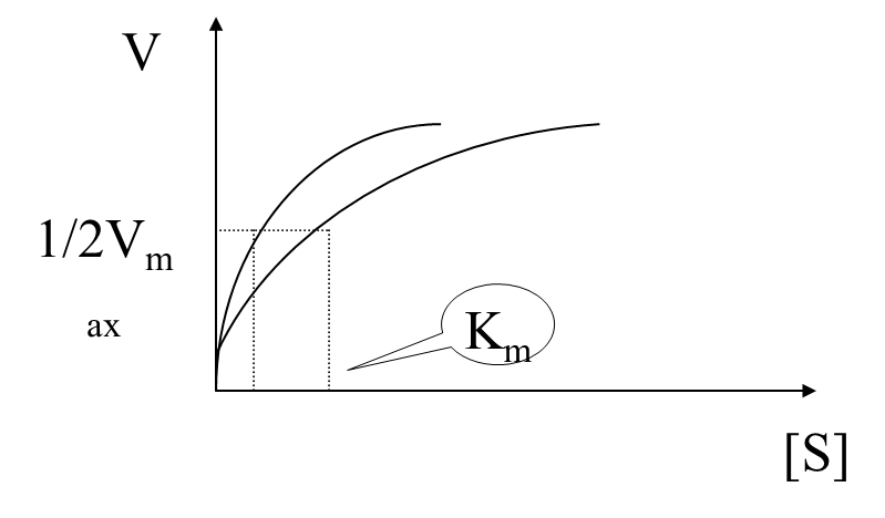
  Every term in this expression is constant for a given enzyme under a specified set of conditions. The resulting K_m is therefore characteristic of the enzyme–substrate pair under those conditions. It depends on the enzyme and the identity of the substrate, but not on enzyme concentration.

• (2) An enzyme with broad substrate specificity has a different K_m for each substrate. The substrate with the smallest value is the enzyme’s preferred substrate. For chymotrypsin, for example, that substrate is benzoyltyrosinamide.

  Why? K_m is the substrate concentration that produces half the maximum rate. A smaller K_m means that less substrate is needed to approach saturation and that the rate responds more strongly to a unit change in substrate concentration; in other words, v is more sensitive to Δs.

  Comparing the two derivations reveals another useful relationship.

  Consider the reaction:

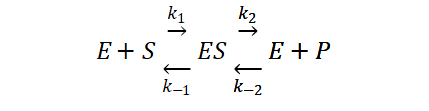
  In the rapid-equilibrium model, the equilibrium constant K_s is:

  In the steady-state model, the Michaelis constant K_m is:

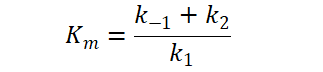
  Comparing the two expressions:

  When k₁ ≫* k₂*, so that ES → P + E is an extremely slow step in the overall reaction:

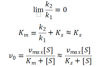
  Thus, the rapid-equilibrium model is a special case of the steady-state model. When ES → P + E is extremely slow and k₂/k₁ is very small, the steady-state result approaches the rapid-equilibrium result. Another way to express the relationship is: steady state = rapid equilibrium + slow equilibrium.

IV. Linearizing the Michaelis–Menten Equation

  The Michaelis–Menten equation is the classic biochemical relationship between the initial substrate concentration and the rate of an enzyme-catalyzed reaction. Fitting its hyperbolic curve can introduce substantial error, so the equation is often rearranged into a linear form. Common methods include the Lineweaver–Burk double-reciprocal plot, Eadie–Hofstee plot, Hanes–Woolf plot, and Eisenthal plot. Of these, the Lineweaver–Burk plot is the most widely used.

  Hans Lineweaver and Dean Burk proposed the double-reciprocal plot in 1934. It is obtained by taking the reciprocal of both sides of the Michaelis–Menten equation and rearranging:

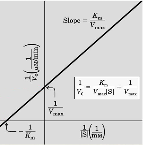
  The plot provides direct estimates of the two key Michaelis–Menten parameters and can also be used for inhibited reactions. Its weakness is the uneven distribution of data: points cluster in the lower-left portion of the line, while reciprocation greatly magnifies errors at low substrate concentrations. Those points may lie far from the fitted line and reduce the accuracy of both parameter estimates. Eadie–Hofstee and Hanes–Woolf plots can mitigate the large errors of the Lineweaver–Burk method at very low or very high substrate concentrations.

V. The Michaelis–Menten Equation under Reversible Inhibition

  An inhibitor reduces or abolishes enzyme activity by acting on an essential functional group without denaturing the protein. The result may resemble denaturation, but the mechanisms are fundamentally different. Denaturation disrupts the interactions that maintain an enzyme’s conformation, including hydrogen bonds, hydrophobic interactions, van der Waals forces, and sometimes disulfide bonds. The enzyme then loses its three-dimensional structure and biological activity. Inhibition instead targets particular reactive groups. Diisopropyl fluorophosphate, for example, forms a phosphate ester bond with an active-site hydroxyl group in proteases and esterases, blocking normal catalysis. Organomercury compounds and halogenated alkylating agents can similarly react with sulfhydryl groups.

  The enzyme’s overall conformation remains intact during inhibition; only particular functional groups are modified, reducing its activity.

  Inhibition can be irreversible or reversible, depending on how tightly the inhibitor binds to the enzyme. Reversible inhibition is further divided into competitive, noncompetitive, and uncompetitive inhibition.

(1) Competitive inhibition

  As the name suggests, a competitive inhibitor competes with the substrate for the enzyme’s active site. It binds reversibly to free enzyme to form an enzyme–inhibitor complex. By occupying the active site, it prevents substrate binding and lowers the reaction rate.

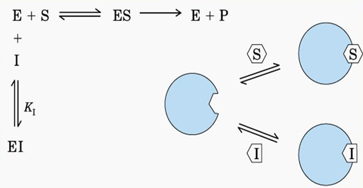
  Competitive inhibitors often resemble the substrate. Malonate, for example, competes with succinate for the active site of succinate dehydrogenase. The enzyme may mistake the inhibitor for its substrate, or steric hindrance may block normal substrate binding. Once bound to the inhibitor, the enzyme can neither accept the correct substrate nor catalyze the reaction. In effect, less enzyme remains available, so the observed activity falls.

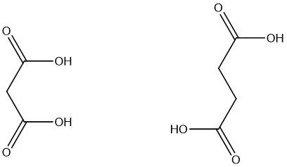
  Succinic acid, also known as butanedioic acid or ethane-1,2-dicarboxylic acid, has the molecular formula C₄H₆O₄. Succinate dehydrogenase converts it to fumaric acid.

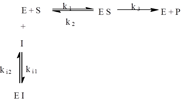
  Competitive inhibition can be treated as two simultaneous reactions involving enzyme E:

  The reactions proceed in parallel. Increasing the concentration of substrate S shifts the equilibrium of

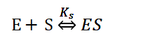
  to the right, while the reaction

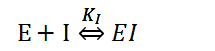
  is suppressed. A high enough [S] can therefore overcome the effect of inhibitor I.

  The rate equation is derived as follows:

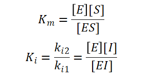
  Substitute

  into the expression for K_i to obtain:

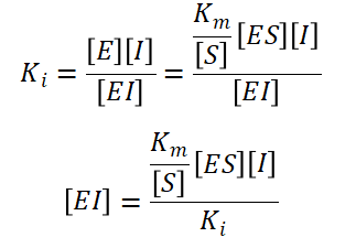
  From the Michaelis hypothesis:

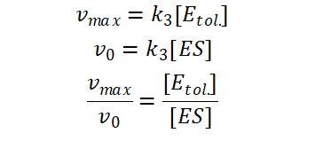
  Substitute into the enzyme-conservation equation

  to obtain:

  Substitute into

  to obtain:

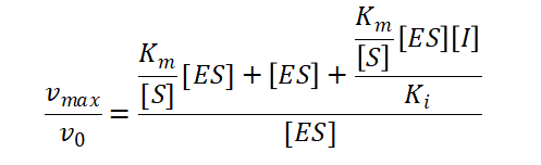
  Rearranging gives:

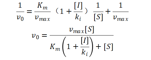
  The equations show that competitive inhibition increases with inhibitor concentration [I] and decreases with substrate concentration [S]. At fixed [I] and [S], inhibition is stronger when K_i is smaller and K_m is larger.

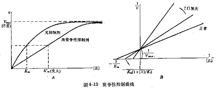
  The Lineweaver–Burk plot shows the defining kinetic pattern of competitive inhibition: the maximum rate v_max remains unchanged, while the apparent Michaelis constant K_m increases.

(2) Noncompetitive inhibition

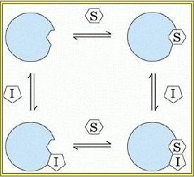
  A noncompetitive inhibitor binds outside the active site and changes the enzyme’s conformation so that it can no longer catalyze product formation. It can bind either free enzyme or the enzyme–substrate complex, forming a ternary EIS complex. The inhibitor does not prevent substrate binding, but it keeps the enzyme–substrate complex from proceeding to product. Some heavy-metal ions, including Cu²⁺, Pb²⁺, and Hg²⁺, act in this way.

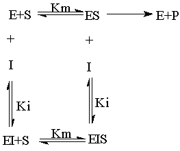
  From

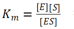
  we obtain:

  Similarly, from

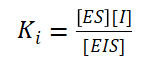
  we obtain:

  From

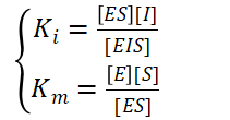
  solving gives:

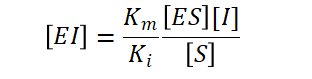
  Substitute the preceding results into:

  Rearranging gives:

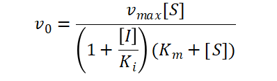
  The double-reciprocal equation is:

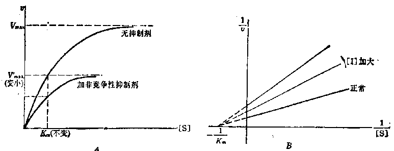
  The Michaelis–Menten equation for noncompetitive inhibition shows that the degree of inhibition depends only on inhibitor concentration [I] and K_i, not on substrate concentration [S] or the substrate’s Michaelis constant K_m. The graph shows that K_m remains unchanged.

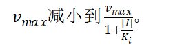
(3) Uncompetitive inhibition

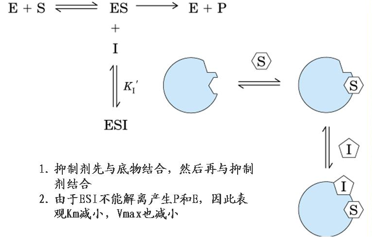
  Unlike a competitive inhibitor, an uncompetitive inhibitor binds only to the enzyme–substrate complex. The resulting ternary complex cannot release product, so both the effective enzyme concentration and the observed activity fall. This mechanism is common in multisubstrate reactions.

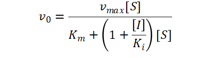
  The rate equation is:

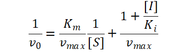
  The double-reciprocal equation is:

  The derivation follows the same general steps as the competitive case and is omitted here.

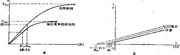
  Uncompetitive inhibition decreases v_max and K_m in the same proportion, producing a family of parallel lines. Its strength depends on K_i, K_m, [S], and [I], and is directly proportional to both [S] and [I]. At fixed [I] and [S], inhibition becomes weaker as either K_i or K_m increases.

  P.S. Reposting or excerpting this article without the author’s permission is prohibited.