A deterministic comparison-based sorting algorithm requires $\Omega(n\lg n)$ comparisons on its worst-case input. But how many comparisons does a randomized algorithm make in expectation on its worst-case input? This article introduces Yao’s principle and uses it to derive a lower bound for randomized sorting.

Author: silverxz
Reviewed by: phy东西

Introduction

The $\Omega(n\lg n)$ lower bound on the worst-case number of comparisons made by a deterministic comparison-based sorting algorithm is a classic result. It appears in textbooks such as Introduction to Algorithms and in most algorithms courses, so many readers will already know it. (This article assumes only an introductory knowledge of algorithms and probability theory. Following the usual convention in algorithms, lg uses base $2$ .)

But how many comparisons does a randomized algorithm make in expectation on its worst-case input?

If you have never encountered randomized algorithms, you may suspect that allowing randomness cannot magically make an algorithm better. Yet some randomized algorithms really do seem magical.

Quicksort is one example. If it chooses pivots by a fixed rule, ordinary quicksort can take $\Theta(n^2)$ time on its worst-case input. Choosing pivots at random, however, keeps its expected complexity at $O(n\lg n)$ even on the worst input. That may not seem magical enough, since plenty of other sorting algorithms run in $\Theta(n\lg n)$ . A more striking example is Freivalds’ algorithm. It has nothing to do with sorting, but it is so concise and ingenious that it deserves a brief introduction. The algorithm solves the following problem.

Problem: Given three $n\times n$ matrices $A,B,C$ , determine whether $AB$ equals $C$ . In other words, verify whether a matrix multiplication result is correct.

The most direct approach is, of course, to multiply $A$ and $B$ , then check whether $AB$ equals $C$ . Its computational cost is that of matrix multiplication, or $O(n^3)$ by the naive method. It is hard to imagine doing better than matrix multiplication itself, yet Freivalds found a randomized method that astonishes almost everyone who encounters it for the first time.

Lemma (Freivalds’ algorithm)
Let $r\in \{0, 1\}^n$ be a random vector of length $n$ with $01$ entries. Then:
if $AB=C$ , then $ABr=Cr$ always holds;
if $AB\neq C$ , then $\mathrm{Pr}_{r\in \{0, 1\}^n}[ABr=Cr]\leq 1/2$ .

To keep the main text shorter, the proof appears in Note 1. It is quite simple, too.

Using this lemma, choose $k$ independent random vectors $r_1, r_2, \dots, r_k \in \{0, 1\}^n$ . Since multiplying a matrix by a vector takes quadratic time, at a total cost of $O(kn^2)$ we can compute and compare each $ABr_i$ with $Cr_i$ , for $i=1,\dots,k$ . If any pair differs, then $AB\neq C$ . If every pair is equal, the algorithm simply declares that $AB=C$ . By the lemma, the probability of a false result—the actual case is $AB\neq C$ , but every $ABr_i=Cr_i$ and the algorithm is fooled—is at most $2^{-k}$ . When $k$ is fixed as a constant, this is an $O(n^2)$ algorithm.

The fastest matrix-multiplication algorithms known today are still a long way from $O(n^2)$ , yet Freivalds’ remarkably simple method sidesteps matrix multiplication altogether. The price is a small probability of error, but that is easy to manage: repeat the test a few more times. The error probability falls exponentially and soon becomes smaller than the chance of hardware failure, system failure, or the server room exploding (Note 2).

Does this example make randomized algorithms seem more powerful? Many of them solve, with remarkable simplicity, tasks that are much less straightforward for deterministic algorithms. Similar ideas underlie various hashing algorithms and their extensions, including the Bloom filter, which you may have heard of. In essence, they construct a random “fingerprint” as cheaply as possible, then use it to identify or compare objects as reliably as possible.

This does not mean that randomized algorithms truly have better asymptotic complexity than deterministic ones. In the case of Freivalds’ algorithm, we do not know whether an $O(n^2)$ deterministic matrix-multiplication algorithm exists. In theory, one might. It would give us an $O(n^2)$ deterministic test for whether $AB$ equals $C$ , putting the randomized and deterministic algorithms on equal footing. Even if such an algorithm exists, however, it would surely be extremely complicated. The randomized algorithm we just saw is remarkably simple, and that is what makes randomized algorithms so impressive.

Now return to sorting. Could a randomized algorithm somehow beat the deterministic lower bound, using fewer than $\Omega(n\lg n)$ comparisons in expectation on its worst-case input? There is no need to keep you in suspense: the answer is still no. To prove it, we need a tool for establishing lower bounds on randomized algorithms, one that shows even randomization cannot work unlimited miracles.

Yao’s Principle

The tool we will introduce is Yao’s minimax principle, usually shortened to Yao’s principle. It comes from Andrew Yao’s 1977 work and is one of the oldest and most fundamental tools for lower-bound analysis of randomized algorithms. Its central idea is to view the relationship between an algorithm and its input as a game.

You may not know what a “game” means in this context, so consider a familiar example: rock–paper–scissors. Let $\mathcal{A},\mathcal{X}$ be sets and $l$ a binary function on them, defined as follows:

$\mathcal{A}=\mathcal{X}=\{\text{rock, scissors, paper}\}, l(a,x)=\{\text{win, lose, tie}\}$

The game of rock–paper–scissors has two players, whom we will call Alice and Bob. They choose an element from $\mathcal{A}$ and $\mathcal{X}$ , respectively, and those choices determine the outcome. In game-theoretic language, the elements of $\mathcal{A}$ are Alice’s strategies (Note 3), while the elements of $\mathcal{X}$ are Bob’s strategies. Once they have chosen, the function $l$ gives the payoff or cost associated with that pair of strategies.

What does this have to do with algorithms? For the sorting problem, let $\mathcal{A}$ be the set of all deterministic comparison-based sorting algorithms, $\mathcal{X}_n$ the set of all inputs of size $n$ , and $l(a,x)$ the number of comparisons algorithm $a\in \mathcal{A}$ needs to sort input $x\in \mathcal{X}_n$ . Alice and Bob are still playing a game. Think of Alice as the algorithm designer and Bob as an adversary: Alice wants to choose the best possible algorithm $a$ and make $l(a,\cdot)$ as small as possible, while Bob wants to choose the worst possible input $x$ and make $l(\cdot,x)$ as large as possible.

A worst-case analysis of a particular algorithm $a\in \mathcal{A}$ —for example, the number of comparisons that a sorting algorithm $a\in \mathcal{A}$ makes in the worst case—allows Bob to attack $a$ with the worst input $x$ . The maximum number of comparisons can be written as

$\max_{x\in \mathcal{X}_n} l(a, x)$

From this game-theoretic perspective, the familiar $\Omega(n\lg n)$ lower bound says that no matter which algorithm $a$ Alice chooses, Bob can use his knowledge of $a$ to find a sufficiently bad input $x$ on which algorithm $a$ requires $l(a,x)>cn\lg n$ comparisons. Notice the order of play: Alice chooses the algorithm first, and Bob, knowing her choice, can tailor his attack. In symbols, there is a constant $c>0$ such that, for all sufficiently large $n$ ,

$\min_{a\in \mathcal{A}}\max_{x\in \mathcal{X}_n} l(a,x) > cn\lg n$

The left-hand side is the number of comparisons required by the best algorithm on its worst input of size $n$ . Observe how the expression captures the order just described. If we add parentheses, it becomes

$\min_{a\in \mathcal{A}} \Big( \max_{x\in \mathcal{X}_n} \big(l(a,x)\big) \Big)$

The inner $\max_{x\in\mathcal{X}_n}$ operates on the value $a\in \mathcal{A}$ selected by the outer operation and, for this $a$ , chooses the input that maximizes $l(a, x)$ . In other words, Bob knows $a$ before maximizing $l(a, x)$ , which captures the order of play. This point matters because we will repeatedly encounter interleaved $\min$ and $\max$ operations.

So far, we have only restated the familiar result for deterministic algorithms in different language. With a little time, it should be straightforward to follow.

We have viewed the relationship between deterministic algorithms and inputs as a game. The crucial next question is: what about randomized algorithms?

First consider what a randomized algorithm is. Unlike a deterministic algorithm, it can generate random numbers and make decisions according to their values.

If we fix every random number it generates, a randomized algorithm becomes deterministic. For example, if a C program obtains random numbers with rand, fixing the seed passed to srand fixes the sequence produced by rand. We can therefore regard a randomized algorithm as a random variable whose possible values are deterministic algorithms.

If that last sentence sounded obscure, remember that a random variable need not take numerical values. Drawing one card uniformly at random from a deck defines a random variable whose possible values are the cards and whose distribution is uniform. Similarly, a randomized algorithm selects one algorithm from a set of deterministic algorithms, so it is a random variable taking values in that set. Put more plainly, a randomized algorithm randomly chooses one algorithm from a collection of deterministic algorithms. We will need this probabilistic formulation below, so it is worth taking a moment to understand it.

In mathematical language, let $\Delta(\mathcal{A})$ denote the set of all probability distributions over $\mathcal{A}$ . An element $R\in \Delta(\mathcal{A})$ is therefore a probability distribution, and a randomized algorithm is a random variable following some distribution $R\in \Delta(\mathcal{A})$ , written $A\sim R$ (Note 4).

Return to the contest between Alice and Bob. We now allow Alice to choose a randomized algorithm. She no longer has to commit to a single fixed algorithm $a\in \mathcal{A}$ and let Bob exploit the weaknesses of $a$ . Instead, she can choose a random variable over $\mathcal{A}$ , denoted by $A$ . This randomized algorithm makes Bob’s attack more difficult.

That description alone may not make the benefit obvious, so return to rock–paper–scissors. If Alice can use only a deterministic strategy, Bob always wins. The order of play means that Bob effectively watches Alice make her move before choosing his own. If Alice can instead use a randomized strategy, choosing rock, paper, or scissors with probability $1/3$ each, Bob can no longer target her choice.

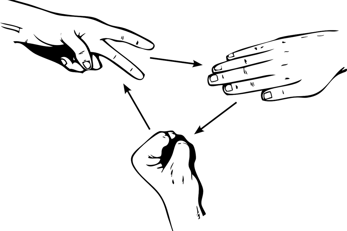
This example shows why a randomized algorithm can have an advantage. The order of play has not changed: Bob can still know Alice’s strategy in advance. But because the strategy itself is random, knowing that “Alice chooses uniformly among rock, paper, and scissors” gives him no way to counter it.

We already know that the worst-case number of comparisons made by the best deterministic sorting algorithm can be expressed as

$\min_{a\in \mathcal{A}}\max_{x\in \mathcal{X}_n} l(a,x)$

What, then, is the expected number of comparisons made by the best randomized algorithm on its worst-case input? Since Alice can choose an algorithm at random, the variable beneath $\min$ is no longer $a\in\mathcal{A}$ but

$\min_{R\in \Delta(\mathcal{A})}\max_{x\in \mathcal{X}_n} \mathbb{E}_{A\sim R}[l(A, x)]$

Alice specifies a randomized strategy $A$ with distribution $R\in\Delta(\mathcal{A})$ . Bob then chooses an input $x\in\mathcal{X}_n$ to attack that strategy, and we calculate its expected cost $\mathbb{E}_{A\sim R}[l(A,x)]$ .

This expression is plainly difficult to evaluate. We do not even know all the deterministic algorithms, much less every distribution $R$ over them. Yao’s principle, however, can transfer the randomness from Alice’s side to Bob’s. That makes the problem much simpler, because we know exactly what $\mathcal{X}_n$ contains: all permutations of $1$ through $n$ . We can now state the theorem.

Theorem (Yao’s minimax principle)
Let $\mathcal{A}, \mathcal{X}$ be two finite sets and let $l:\mathcal{A}\times \mathcal{X}\to \mathbb{R}$ . For every random variable over $\mathcal{A}$ , denoted by $A$ , and every random variable over $\mathcal{X}$ , denoted by $X$ ,
$\max_{x\in\mathcal{X}} \mathbb{E}_{A}[l(A,x)] \geq \min_{a\in \mathcal{A}} \mathbb{E}_{X}[l(a,X)]$

Proof
The proof is short, so we will complete it before explaining what the theorem means.
$\begin{aligned} \max_{x\in\mathcal{X}} \mathbb{E}_{A}[l(A,x)] &\geq \mathbb{E}_X \mathbb{E}_A[l(A,X)]\\ &=\mathbb{E}_A\mathbb{E}_X[l(A,X)]\\ &\geq \min_{a\in \mathcal{A}} \mathbb{E}_{X}[l(a,X)] \end{aligned}$
The first and last lines use the elementary inequality
$\max_{z\in \mathcal{Z}} f(z) \geq \mathbb{E}_{Z} [f(Z)] \geq \min_{z\in \mathcal{Z}} f(z)$
The maximum is at least the average, which is at least the minimum. Straightforward, isn’t it? Such a basic inequality rarely yields anything useful by itself. The crucial step here is exchanging the order of expectation in the second line. The theorem assumes that $\mathcal{A},\mathcal{X}$ are finite, so these expectations are finite double sums whose order can be exchanged. That completes the proof.
In fact, the proposition does not require both sets $\mathcal{A}, \mathcal{X}$ to be finite. Finiteness was used only to exchange the expectations in the second step, and it is enough for one of the two sets to be finite, because a finite sum and an integral can be interchanged. The lower-bound proof for sorting later in this article actually uses this version, in which one set is infinite and the other finite. Writing it as a separate theorem would be cumbersome, so we will not do so (Note 5).
If both sets are infinite, conditions such as $l\geq 0$ allow the integrals to be exchanged using Tonelli’s theorem. Yao’s principle can therefore be extended, but we will not need that version. Readers without a mathematical background can safely ignore it.

The proof is remarkably simple, but the important question is not how the theorem is proved; it is what the theorem tells us. In the statement, $\mathcal{A},\mathcal{X}$ are abstract sets with no assigned meaning, and $l$ is an abstract function. Give them their usual interpretation, and we are back to the game between algorithm designer Alice and adversary Bob. The set $\mathcal{A}$ contains every deterministic algorithm Alice may choose, $\mathcal{X}$ every concrete input Bob may choose, and $l(a,x)$ is the cost incurred by algorithm $a$ on input $x$ , such as its running time or number of comparisons. Alice wants the algorithm that makes $l$ as small as possible; Bob wants the input that makes $l$ as large as possible.

As discussed above, the random variable over $\mathcal{A}$ denoted by $A$ represents one of Alice’s randomized algorithms. The left-hand side, $\max_{x\in\mathcal{X}} \mathbb{E}_{A}[l(A,x)]$ , is Bob’s strongest attack on the randomized algorithm $A$ : he chooses the input with expected cost $\mathbb{E}_{A}[l(A,x)]$ as large as possible, denoted by $x$ . By contrast, the random variable over $\mathcal{X}$ denoted by $X$ represents a randomized input strategy for Bob. Alice chooses the deterministic algorithm with the smallest expected cost against that distribution. The expected cost of this algorithm is the right-hand side, $\min_{a\in \mathcal{A}} \mathbb{E}_{X}[l(a,X)]$ .

Once we understand the two sides, the inequality itself becomes clear. To lower-bound the expected cost of a randomized algorithm $A$ on its worst input—the left-hand side—we may instead analyze the expected cost of the best deterministic algorithm against a random input $X$ —the right-hand side. The latter is a lower bound for the former. More concretely, suppose we want to prove $\max_{x\in\mathcal{X}} \mathbb{E}_{A}[l(A,x)] > n\lg n$ . The inequality tells us that it is enough to prove $\min_{a\in \mathcal{A}} \mathbb{E}_{X}[l(a,X)] > n\lg n$ , after which

$\max_{x\in\mathcal{X}} \mathbb{E}_{A}[l(A,x)] \geq \min_{a\in \mathcal{A}} \mathbb{E}_{X}[l(a,X)] > n\lg n$

Readers who have followed this far may wonder whether this method analyzes only one randomized algorithm $A$ . Our original goal was a lower bound for every randomized sorting algorithm, not merely one particular algorithm. Those sound very different. But the theorem allows arbitrary $A$ and $X$ , so we immediately obtain the following corollary.

Corollary
Let $\mathcal{A}, \mathcal{X}$ be two finite sets and let $l:\mathcal{A}\times \mathcal{X}\to \mathbb{R}$ . Then
$\min_{R\in \Delta(\mathcal{A})}\max_{x\in \mathcal{X}} \mathbb{E}_{A\sim R}[l(A, x)] \geq \max_{D\in \Delta(\mathcal{X})}\min_{a\in\mathcal{A}} \mathbb{E}_{X\sim D}[l(a,X)]$
In particular, for any random input—that is, any random variable over $\mathcal{X}$ , denoted by $X$ —
$\min_{R\in \Delta(\mathcal{A})}\max_{x\in \mathcal{X}} \mathbb{E}_{A\sim R}[l(A, x)] \geq \min_{a\in\mathcal{A}} \mathbb{E}_{X}[l(a,X)]$

Proof
As noted above, $A, X$ in the theorem are arbitrary. Thus,
$\forall R\in \Delta(\mathcal{A}),\quad \max_{x\in \mathcal{X}} \mathbb{E}_{A\sim R}[l(A, x)] \geq \min_{a\in\mathcal{A}} \mathbb{E}_{X}[l(a,X)]$
Since this inequality holds for every $R$ , it still holds for the $R$ that minimizes its left-hand side. Therefore,
$\min_{R\in \Delta(\mathcal{A})}\max_{x\in \mathcal{X}} \mathbb{E}_{A\sim R}[l(A, x)] \geq \min_{a\in\mathcal{A}} \mathbb{E}_{X}[l(a,X)]$
Repeating the same argument for $X\sim D$ gives
$\min_{R\in \Delta(\mathcal{A})}\max_{x\in \mathcal{X}} \mathbb{E}_{A\sim R}[l(A, x)] \geq \max_{D\in \Delta(\mathcal{X})}\min_{a\in\mathcal{A}} \mathbb{E}_{X\sim D}[l(a,X)]$

We have immediately turned a statement about one randomized algorithm $A$ into a statement about all randomized algorithms. The result gives us a standard pattern for lower-bound analysis. To prove that every randomized algorithm has high cost—that $\min_{R\in \Delta(\mathcal{A})}\max_{x\in \mathcal{X}} \mathbb{E}_{A\sim R}[l(A, x)]$ exceeds some value—it is enough to show that, for some random input $X$ , every deterministic algorithm has high cost—that $\min_{a\in\mathcal{A}} \mathbb{E}_{X}[l(a,X)]$ exceeds that value. This is what we mean by transferring randomness from the algorithm to the input.

Some readers may ask: this is only an inequality, and its proof is extremely simple. Is the resulting lower bound genuinely useful, or could it be very loose and utterly trivial?

If that question occurred to you, it is an excellent one. The answer reveals the power of the result. When $\mathcal{A},\mathcal{X}$ are finite, we can in fact prove

$\min_{R\in \Delta(\mathcal{A})}\max_{x\in \mathcal{X}} \mathbb{E}_{A\sim R}[l(A, x)] = \max_{D\in \Delta(\mathcal{X})}\min_{a\in\mathcal{A}} \mathbb{E}_{X\sim D}[l(a,X)]$

The $\max$ is attained, so equality holds. If you can construct the random variable $X$ , or equivalently the distribution $D$ , that attains the maximum on the right, the resulting lower bound is tight: transferring the randomness loses nothing. In practice, finding a sufficiently difficult $X$ is often the hard part of applying Yao’s principle. The harder the distribution you construct, the tighter the lower bound you obtain. Yao’s principle is not a theorem that can be applied mechanically; it often appears only as the final step of a larger proof.

This equality follows directly from the von Neumann minimax theorem in game theory. Its proof is unrelated to our subject, so we will omit it. The equality need not hold in the infinite case. This also explains the name “Yao’s minimax principle.”

A Lower Bound on Comparisons in Randomized Comparison-Based Sorting

We can now answer the question posed at the beginning. First, let us review the basic deterministic result, because we will use the same decision-tree model. The review will be brief; it is only meant as a refresher.

Theorem
The number of comparisons made by a deterministic comparison-based sorting algorithm has a lower bound of $\Omega(n\lg n)$ .

Proof
“Comparison-based” means that the algorithm cannot directly use the specific values of the elements. It can learn their ordering only by asking questions of the form $x_i < x_j\ ?$ . In sorting problems, we ordinarily assume that no two elements are equal.
Consider a deterministic sorting algorithm. Since the algorithm is deterministic, its comparison strategy is completely fixed: which two elements it compares next depends entirely on the outcomes of all earlier comparisons.
We can therefore unfold the algorithm’s entire execution into a binary tree called a decision tree. Each node represents the comparison the algorithm makes when it reaches that point. For example, the root might be $x_i < x_j \ ?$ , meaning that the algorithm begins by comparing $x_i, x_j$ . If the root’s left child is $x_k < x_l\ ?$ , then after finding $x_i < x_j$ , the algorithm next compares $x_k, x_l$ . If the root’s right child is $x_m < x_n\ ?$ , then after finding $x_i > x_j$ , it next compares $x_m, x_n$ . Because the algorithm is deterministic, its behavior uniquely determines the whole tree.
The algorithm follows the left or right child after each comparison and continues downward. When it stops, it makes no further comparisons and has reached a leaf of the decision tree, where it outputs one fixed ordering. Thus, every leaf corresponds to one permutation. If the algorithm is correct, inputs with different orders cannot reach the same leaf; otherwise, at least one of them would receive the wrong output. There are $n!$ possible orders, so the decision tree has at least $n!$ leaves.
Let the decision tree have height $h$ . A binary tree of height $h$ has at most $2^h$ leaves, so
$2^h \geq n!$
By Stirling’s formula,
$h \geq \lg (n!) = n\lg n- O(n) = \Omega(n\lg n)$
The algorithm therefore needs at least $\Omega(n\lg n)$ comparisons to sort the input corresponding to a deepest leaf.

That completes the review. We now want to analyze randomized algorithms, for which the decision-tree model no longer seems applicable. One important reason the model works for deterministic algorithms is that their comparison strategy is fixed. Whenever all previous comparison outcomes are the same, the next pair of elements to compare is fully determined, allowing the execution to be expanded into a binary decision tree. A randomized algorithm breaks this property: its next comparison may itself be chosen at random.

This is precisely where Yao’s principle helps. It shifts the randomness from the algorithm to the input, making the algorithm deterministic again and restoring the decision-tree model. We have laid enough groundwork, so let us proceed directly to the proof.

Theorem
The expected number of comparisons made by a randomized comparison-based sorting algorithm on its worst-case input has a lower bound of $\Omega(n\lg n)$ .

Proof
Recall Yao’s principle: we need a distribution $D$ over random inputs that makes the problem difficult for every deterministic algorithm. We noted that constructing $D$ is often the hard part. Here, however, there is a natural choice that readers have probably already guessed: the uniform distribution. In sorting, all elements and all permutations have equal standing. There is no reason to favor one over another, so trying the uniform distribution is the most natural approach.
Let $\mathcal{A}=$ { all deterministic comparison-based sorting algorithms }, $\mathcal{X}=$ { all permutations of 1 through n }, and let $l(a,x)=$ the number of comparisons algorithm a makes to sort input x. Let $D$ be the uniform distribution over $\mathcal{X}$ . To apply Yao’s principle, we must lower-bound $\min_{a\in A}\mathbb{E}_{X\sim D}[l(a,X)]$ , the expected number of comparisons made by a deterministic algorithm under the uniform distribution. This is precisely what decision trees allow us to analyze.
For a deterministic algorithm $a\in\mathcal{A}$ , consider its decision tree again. The $n!$ distinct inputs reach $n!$ distinct leaves. Let the depths of these $n!$ leaves be $d_1,d_2,\dots,d_{n!}$ . The expected number of comparisons made by $a$ on this random input is the average of all these depths:
$\mathbb{E}_{X\sim D}[l(a, X)]=\frac{1}{n!}\sum_{k=1}^{n!} d_k$
Estimating the right-hand side requires only a little mathematics. First, we have the Kraft inequality
$\sum_{k=1}^{n!} 2^{-d_k} \leq 1$
Do not be alarmed; its intuitive proof is simple. First imagine a full binary tree, in which every node has either two children or none. Assign every leaf at depth $d$ the value $2^{-d}$ . Then repeatedly merge pairs of sibling leaves, as in the game Merge Watermelon: remove two sibling leaves, each worth $2^{-d}$ , and assign their parent, now a new leaf, the value $2^{-d+1}$ . Keep merging until only the root, with value $1$ , remains. Thus, for a full binary tree, the leaf depths satisfy $\sum 2^{-d_i}=1$ . In a binary tree that is not necessarily full, some nodes have only one child. Contract each such edge by merging the node with its only child, making the tree full. That edge only increased the leaf depths, so the original sum on the left can only be smaller. Hence $\sum_{k=1}^{n!}2^{-d_k}\leq1$ .
One final bit of mathematics remains. Jensen’s inequality says that if, on $\mathbb{R}$ , the function $f(x)$ is convex, positive real numbers $a_1,\dots,a_m>0$ satisfy $\sum_{i=1}^m a_i = 1$ , and $x_1,\dots,x_m\in \mathbb{R}$ , then
$f\left(\sum_{i=1}^m a_i x_i\right) \leq \sum_{i=1}^m a_if(x_i)$
We know that $f(x)=2^{-x}$ is convex. Therefore,
$2^{-\frac{1}{n!}\sum_{k=1}^{n!} d_k}\leq \frac{1}{n!}\sum_{k=1}^{n!}2^{-d_k} \leq \frac{1}{n!} \Longrightarrow \mathbb{E}_{X\sim D}[l(a, X)]=\frac{1}{n!}\sum_{k=1}^{n!} d_k \geq \lg n!$
Here $1/n!$ plays the role of $a_i$ in the inequality, and $d_k$ plays the role of $x_i$ . Since the result holds for every algorithm $a$ ,
$\min_{a\in \mathcal{A}}\mathbb{E}_{X\sim D}[l(a, X)]\geq \lg n! = \Omega(n\lg n)$
Yao’s principle now gives
$\min_{R\in \Delta(\mathcal{A})}\max_{x\in \mathcal{X}} \mathbb{E}_{A\sim R}[l(A, x)] \geq \min_{a\in\mathcal{A}} \mathbb{E}_{X\sim D}[l(a,X)] =\Omega(n\lg n)$
In other words, every randomized algorithm $A$ has some sufficiently bad input $x$ on which its expected number of comparisons is also of order $n\lg n$ .

Randomized Sorting Algorithms That May Err

At this point, the problem seems fully resolved, though the answer is a little disappointing: there is no miracle, and randomized algorithms cannot break the $\Omega(n\lg n)$ barrier.

Careful readers may still have a question. Freivalds’ algorithm, our opening example, allows a small probability of error, and that is a major reason for its excellent performance. Although our proof seemed to cover every randomized algorithm, it did not: it covered only algorithms that never err. The randomized algorithm $A$ is a random variable over $\mathcal{A}$ , and $\mathcal{A}$ consists entirely of correct deterministic algorithms. No matter how they are randomized, $A$ therefore never errs either. Could a randomized algorithm become miraculously better if we allowed some probability of error? As an encore, this section answers that question as well. It is slightly more complicated than what came before, but not substantially more difficult.

The preceding analysis missed randomized algorithms that may err because $\mathcal{A}$ did not contain incorrect deterministic algorithms. Our first step should therefore be to enlarge $\mathcal{A}$ so that it includes them.

The problem is that a deterministic algorithm in this larger set may be spectacularly wrong. Consider a simple and rather foolish randomized algorithm: with probability $\varepsilon$ , it returns the input unchanged; with probability $1-\varepsilon$ , it runs a correct deterministic sorting algorithm such as merge sort. This is certainly a randomized sorting algorithm that may err, with an error probability of at most $\varepsilon$ . To include it, $\mathcal{A}$ must contain the “return the input unchanged” algorithm, which is wrong almost all the time. Yet that algorithm makes no comparisons at all. If it belongs to $\mathcal{A}$ , then

$\min_{a\in \mathcal{A}}\mathbb{E}_{X\sim D}[l(a, X)]=0$

which tells us nothing.

The underlying problem is that we want to control the randomized algorithm’s error probability, and the comparison bound should depend on that probability. Yet a randomized algorithm with bounded error may still be a distribution over deterministic algorithms that are wildly inaccurate, while our cost function $l$ records only the number of comparisons and says nothing about error.

The framework of Yao’s principle allows only one function $l$ , so we seemingly cannot use separate functions for comparison cost and error. What can we do? Readers familiar with optimization may recognize a standard device: Lagrangian relaxation. This technique lets us combine two quantities that we want to optimize subject to a joint constraint.

Let $\mathcal{A}$ be the set of all deterministic algorithms, whether or not they sort correctly. Leave $\mathcal{X}$ unchanged as the set of all inputs of size $n$ , namely the $n!$ permutations. Redefine $l$ using a parameter $\lambda>0$ :

$l(a, x) = c(a, x) + \lambda e(a, x)$

Here $c(a,x)$ is our original $l(a,x)$ , the number of comparisons made by algorithm $a$ on input $x$ , while $e(a,x)$ is defined by

$e(a, x)= \begin{cases} 1, & \text{sorting result is incorrect}, \\ 0, & \text{sorting result is correct}. \end{cases}$

Thus, the comparison count $c$ and the error indicator $e$ are combined using the coefficient $\lambda$ in $l$ . Saying that the error probability is at most $\varepsilon$ for a randomized algorithm $A$ means that it satisfies

$\forall x\in\mathcal{X}, \ \mathrm{Pr}_{A}[e(A,x)=1]\leq \varepsilon$

Let us apply the same Yao’s-principle analysis to these definitions of $\mathcal{A},\mathcal{X}, l$ .

Again choose the uniform distribution over $\mathcal{X}$ , denoted by $D$ , and consider a deterministic algorithm $a \in\mathcal{A}$ under this random input. Suppose algorithm $a$ correctly sorts, among all $N=n!$ inputs, a fraction $q$ ; that is, it correctly sorts $qN$ of them.

The case $q=0$ creates a minor nuisance, so first exclude algorithms that are wrong on every input. A better option always exists: an algorithm that outputs one fixed permutation without making any comparisons is still correct for exactly one input. We may therefore discard the case $q=0$ and assume $q>0$ .

Following the earlier decision-tree argument, to sort these $qN$ distinct inputs correctly, the $qN$ inputs must reach different leaves. The tree therefore has at least $qN$ distinct leaves. Let the depths of these $qN$ distinct leaves be $d_1,\dots,d_{qN}$ . The Kraft inequality still holds, so the same Jensen’s-inequality argument gives their average depth:

$\frac 1 {qN}\sum_{k=1}^{qN} d_k \geq \lg (qN)$

The details are left for the reader to verify. It follows that

$\begin{aligned} \mathbb{E}_{X\sim D}[l(a, X)] &= \frac 1 N \sum_{x\in X} l(a, x)\\ &= \frac 1 N \left( \sum_{x\text{ can be sorted correctly}} l(a, x)+ \sum_{x\text{ cannot be sorted correctly}} l(a, x) \right)\\ &\geq \frac 1 N \left( \sum_{x\text{ can be sorted correctly}} c(a, x)+ \sum_{x\text{ cannot be sorted correctly}} \lambda e(a, x) \right)\\ &= \frac 1 N \left( \sum_{k=1}^{qN}d_k + \sum_{x\text{ cannot be sorted correctly}} \lambda \right)\\ &\geq \frac 1 N \big( qN\lg (qN) + \lambda(N-qN) \big)\\ &= q\lg(qN)+\lambda(1-q) \end{aligned}$

Notice that this bound depends only on $q$ and ignores every other feature of the algorithm. In effect, it reduces the complexity of the algorithm set $\mathcal{A}$ . We no longer need to consider every $a\in\mathcal{A}$ individually; we need only consider the fraction of inputs it sorts correctly, $q=1/N,2/N,\dots,1$ . Applying Yao’s principle, for every randomized algorithm $A$ we have

$\max_{x\in \mathcal{X}} \mathbb{E}_{A}[l(A, x)] \geq \min_{a\in\mathcal{A}} \mathbb{E}_{X\sim D}[l(a,X)] \geq \min_{q=\frac 1 N, \dots, 1} (q\lg(qN)+\lambda(1-q))$

The left-hand side is not yet what we want, because $l$ now combines the number of comparisons with the cost of error. Let $A$ be a randomized algorithm whose error probability is at most $\varepsilon$ , so that

$\forall x\in\mathcal{X},\ \mathrm{Pr}[e(A,x)=1] \leq \varepsilon$

The definition of $l$ then gives

$\max_{x\in \mathcal{X}} \mathbb{E}_{A}[l(A, x)] \leq \max_{x\in \mathcal{X}} \mathbb{E}_{A}[c(A, x)] + \lambda\varepsilon$

Rearranging and substituting the inequality from Yao’s principle yields

$\max_{x\in \mathcal{X}}\mathbb{E}_{A}[c(A, x)] \geq \min_{q=\frac 1 N, \dots, 1} \big(q\lg(qN)+\lambda(1-\varepsilon-q)\big)$

This is the form we wanted. It says that, with error probability at most $\varepsilon$ , a randomized algorithm $A$ makes at least the quantity on the right in expected comparisons on its worst-case input.

This is not yet the final result, because the expression still contains $\lambda$ . It holds for every $\lambda>0$ , so we want to choose $\lambda$ to maximize the right-hand side and make the inequality as tight as possible. In other applications, we would normally differentiate with respect to $\lambda$ and find the maximum. Here, the inner $\min$ makes direct differentiation awkward. A geometric treatment could interpret the expression through an upper convex hull, but explaining that approach would take some work, and readers may not know what a convex hull is. We will take the bluntest route and calculate it directly.

First, $q$ takes the discrete values $1/N, 2/N, \dots, 1$ , which is inconvenient. For a given $\lambda$ , we plainly have

$\min_{q=\frac 1 N, \dots, 1} \big(q\lg(qN)+\lambda(1-\varepsilon-q)\big) \geq \min_{0<q\leq 1} \big(q\lg(qN)+\lambda(1-\varepsilon-q)\big)$

We may therefore work with the continuous case and still obtain a lower bound. Define

$f(\lambda) = \min_{0<q\leq 1} \big( q\lg(qN)+\lambda (1-\varepsilon-q) \big)$

We begin with the inner minimum. For fixed $\lambda>0$ , define

$g(q) = q\lg (qN) + \lambda(1-\varepsilon-q)$

Differentiating—and remembering that our $\lg$ has base $2$ —gives

$g'(q)=\lg (qN) + \lg e -\lambda$

The minimum is therefore attained at the critical point $q=\frac{1}{eN}2^\lambda$ . Because, in $f(\lambda)$ , the $\min$ restricts $q$ to $(0, 1]$ , we need a short case analysis. When $0 < \lambda \leq \lg (eN)$ , the minimizer $q=\frac{1}{eN}2^\lambda \leq 1$ lies within the interval. When $\lambda > \lg (eN)$ , for $q<1$ the derivative $g'(q)<0$ , so the minimum occurs at $q=1$ . Substituting into $f(\lambda)$ gives

$f(\lambda)= \begin{cases} -\frac{\lg e}{eN}2^\lambda + \lambda(1-\varepsilon), & 0 < \lambda \leq \lg (eN) , \\ \lg N - \lambda \varepsilon, & \lambda > \lg (eN). \end{cases}$

This removes the outer $\min$ . We want to maximize $f$ . Direct calculation verifies continuity at the breakpoint, where $f(\lg (eN))=(1-\varepsilon)\lg N - \varepsilon \lg e$ . Since, when $\lambda > \lg(eN)$ , $f$ decreases monotonically, we can discard the part with $\lambda > \lg (eN)$ while finding the maximum and consider only $0 < \lambda \leq \lg(eN)$ .

Differentiating $f$ gives

$f'(\lambda) = -\frac{1}{eN}2^{\lambda} + (1-\varepsilon)$

The maximum occurs at the critical point $\lambda = \lg(eN(1-\varepsilon)) \leq \lg(eN)$ . One boundary issue remains. If $\lambda > 0$ , substituting it into $q=\frac{1}{eN}2^\lambda$ gives $q=1-\varepsilon$ , and then $f(\lambda)=(1-\varepsilon)\lg((1-\varepsilon)N)$ . If $\lambda < 0$ , then $(1-\varepsilon)\lg((1-\varepsilon)N)$ is less than $0$ and remains a valid, though trivial, lower bound on the number of comparisons, which is always nonnegative. We may therefore use the same bound without compromising correctness.

Returning to the result derived above, we can finally write

$\max_{x\in \mathcal{X}}\mathbb{E}_{A}[c(A, x)] \geq (1-\varepsilon)\lg((1-\varepsilon)N)$

We have proved the following theorem.

Theorem
If a randomized comparison-based sorting algorithm $A$ has error probability at most $\varepsilon < 1$ , then for every positive integer $n$ , there is an input of size $n$ on which the expected number of comparisons made by $A$ is at least $(1-\varepsilon)\lg ((1-\varepsilon)n!)$ .

For a constant error probability, this quantity is still of order $\Omega(n\lg n)$ . Thus, even randomized sorting algorithms that may err cannot break this lower bound.

Interestingly, achieving the factor $1-\varepsilon$ is extremely simple. Consider the foolish algorithm mentioned earlier: with probability $\varepsilon$ , it produces a random, probably incorrect ordering; with probability $1-\varepsilon$ , it runs a deterministic sorting algorithm. This produces a randomized algorithm whose expected comparison count is of order $(1-\varepsilon)\lg (n!)$ . Randomization truly offers little extra leverage in sorting. This concludes our use of Yao’s principle to analyze randomized algorithms through the example of sorting.

Conclusion

This article has introduced Yao’s principle and used it to analyze randomized sorting algorithms. Now that we have reached the end, you may feel that we used no advanced mathematics, devised no ingenious algorithm, and proved the central theorem with an argument so simple that it seemed almost trivial. Some readers may find that disappointing.

Yet many important results matter not because they are abstruse or technically intricate, but because they offer a fresh and clarifying point of view. The heart of Yao’s principle is not its two-line proof; it is the insight that an algorithmic problem can be viewed as a game. Once that insight gives us the right structure, the theorem follows naturally, and the resulting theory is concise and elegant.

As noted above, this result is due to Andrew Yao. Born in 1946, Professor Yao received the Turing Award in 2000. One reason for choosing this topic is that December 24 this year will be his eightieth birthday. We wish him good health.

Remarks

This section collects proofs omitted from the main text and additional comments on some of its content. A few notes require more mathematical background than the main article; read them as needed.

Note 1. We prove the lemma stated in the main text.

Proof
If $AB=C$ , then plainly $ABr=Cr$ . We prove that if $AB\neq C$ , then $\mathrm{Pr}_{r\in \{0, 1\}^n}[ABr=Cr]\leq 1/2$ .
If $AB\neq C$ , then $D=AB-C$ is not the all- $0$ matrix and must contain a nonzero entry. Suppose this entry $d_{i,j}$ lies in row $i$ , column $j$ . If vector $r$ has its $j$ th component changed from $0$ to $1$ , then the $ABr-Cr=Dr$ vector has its $i$ th component increased by $d_{i, j}\neq 0$ ; conversely, changing it from $1$ to $0$ decreases that component by $d_{i,j}$ . Thus, when every other component of $r$ is fixed, at least one of the two possibilities for the $j$ th component, $0$ or $1$ , satisfies $ABr\neq Cr$ . Therefore,
$\mathrm{Pr}_{r\in \{0, 1\}^n}[ABr=Cr]\leq 1/2$

Note 2. Randomized algorithms with bounded running time and a small probability of error are called Monte Carlo algorithms. They have no connection to Monte Carlo sampling beyond sharing a name derived from Monte Carlo and its famous casino. As discussed in the main text, repeating the algorithm reduces its error probability exponentially.
By contrast, randomized algorithms that never err but have random running times are called Las Vegas algorithms, after the gambling city of Las Vegas. A Las Vegas algorithm always returns a correct result. Its expected running time is usually required to be bounded, but its worst-case running time need not be. For certain random sequences, it may run for a very, very long time. Imagine an extremely foolish sorting algorithm that randomly shuffles the data, checks whether they are sorted, and, if not, repeats: shuffle, check, and so on until the random shuffle happens to put the data in order. This is a Las Vegas algorithm. If it halts, the data are certainly sorted; but it may also run forever and never halt.
Note 3. Strictly speaking, the strategies described here are called pure strategies in game theory, meaning deterministic strategies. The randomized strategies discussed later are called mixed strategies. As explained in the main text, a mixed strategy is a random variable over pure strategies.
Note 4. A randomized algorithm can be regarded as a random variable, but strictly speaking, a random variable need not be a randomized algorithm because its distribution may not be sampleable. This raises minor computability issues. Similar issues mean that our later discussion of whether the bound from Yao’s principle is tight applies more directly to the game model and may leave a small gap between that model and an actual algorithm. This almost never causes a real problem. Readers unfamiliar with the issue can ignore it, and we will not draw a strict distinction here.
Note 5. Strictly speaking, when a set becomes infinite, a maximum or minimum need not be attained; values may only approach it arbitrarily closely. Mathematics handles this by replacing $\max,\min$ , which denote maxima and minima, with $\sup,\inf$ , which denote suprema and infima. Because this article assumes no mathematical background, introducing those new concepts would add unnecessary cognitive load. The distinction also makes little difference here, so the main text sacrifices a little rigor and continues to use $\max,\min$ , including in the proof of the sorting lower bound.