A Few Simple Thoughts Inspired by a Rolling Spring
Author: phy Dongxi
(A text-heavy piece of popular science—consider yourself warned.)
Most of us played with springs as children—those in retractable pens, for example, or in a Rubik’s Cube (yes, I really do bring up the Rubik’s Cube every three sentences). Helical springs like these turn up everywhere:

Roll one of these springs across a tabletop, and you seem to see a train of waves traveling from one end to the other. A rotating drill bit or the red, white, and blue pole outside a barbershop creates the same illusion: the spiral seems to keep “emerging” from one end and disappearing at the other. It certainly looks like a wave on the move.
We can calculate this wave’s speed quite easily. Suppose the helix has radius r, rotational frequency f, and pitch h. What we see as a “wave” is the helix’s projection onto a plane parallel to its central axis, as shown below:
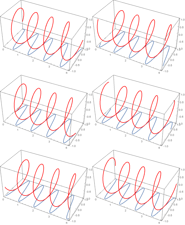
During one period, 1/f, the wave “advances” by one pitch h, so its speed is hf. Meanwhile, a point on the helix circles the central axis at a speed of 2πrf. Compare the two, and you find that whenever h>2πr, the wave’s apparent speed can exceed the speed of light even though no point on the helix does.
Excellent! The whole edifice of physics comes crashing down… or does it?
No. This wave carries no information. Every point follows a predetermined path, much like the spectators in a stadium wave; the result only looks like a traveling wave.
Could we use a more elaborate helix instead? Yes, as the next two figures show:
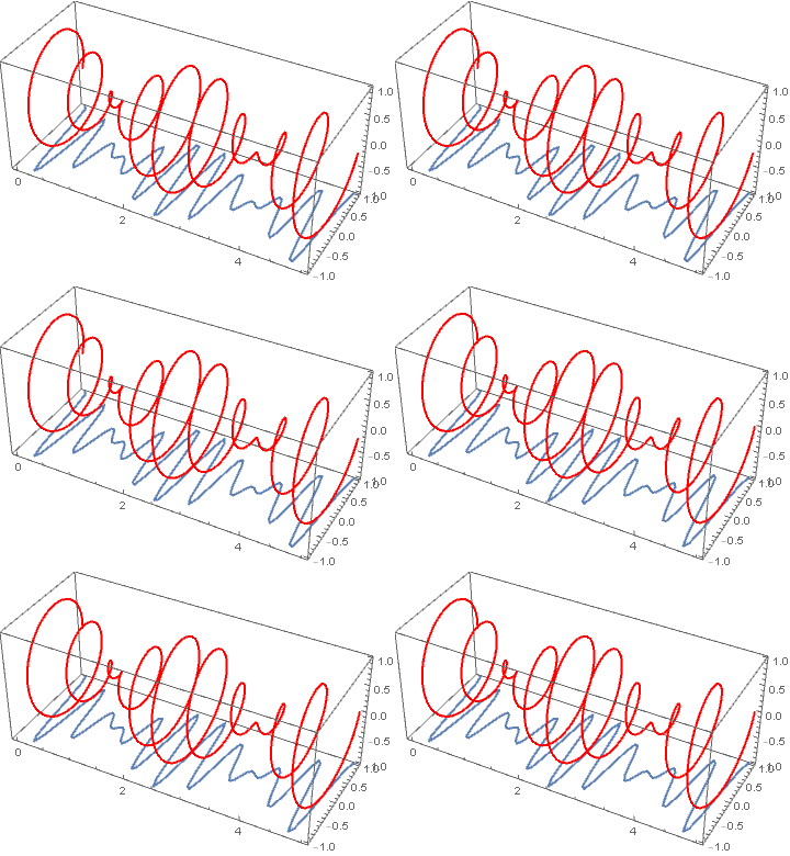
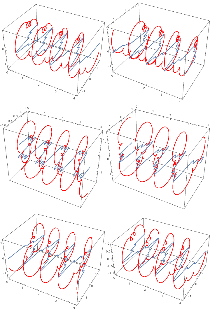
The blue curve is the projection of the red one. Points of equal phase, represented here by successive extrema, keep moving to the right; this is the phase velocity. The helix itself, however, merely rotates in place, and the wave’s complex envelope—the helix’s “outer contour”—does not advance. The speed at which the overall envelope moves can be regarded as the group velocity, the speed at which the waveform as a whole propagates.
The following figure makes the idea easier to visualize:
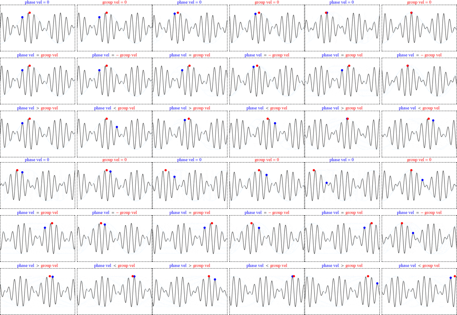
For example, consider two very close angular frequencies, ω1 and ω2, with ω1,ω2≈ω. The two waves satisfy cos(ω1t-k1x)+cos(ω2t-k2x)=2cos(ωt-kx)cos[(ω1-ω2)t/2-(k1-k2)x/2]. The first, high-frequency factor is the carrier moving forward, while the second, much more slowly varying factor describes the propagation of the wave’s shape.
For the full derivation, see Section 48 of The Feynman Lectures on Physics, Vol. I.
Now suppose we treat a given signal as the projection of some helix. Can we reconstruct the corresponding “helix”? That is precisely what the Hilbert transform does. It is a fairly involved integral transform—and an improper integral at that—so in some cases it must be evaluated as a Cauchy principal value. In shorthand, it is the convolution of the original signal with 1/πt.
The Hilbert transform has even broader applications in communications. Once we have a signal’s complex envelope, we can convert a bandpass signal and system into an equivalent baseband signal and system. Because that discussion requires a foundation in Fourier transforms, we will leave it there for now.
For a detailed treatment of its applications, see Chapter 2 of Principles of Communication by Zhou Jiongpan et al., published by Beijing University of Posts and Telecommunications Press.
 爱发电(点击图片跳转)